Presentation Summary
Background & Introduction
Implementation
Software Organization
How to Use
Additional Features/Extension
Impact and Inclusivity
Future Work & Other Possible Extensions
Background & Introduction to Awesome Automatic Differentiation
What is Automatic Differentation?
- A fast and easy derivative method that avoids the use of hyperparamters and iteration.
- Uses dual numbers to compute within machine precision exact derivatives based on elementary primitives
Why is it Useful?
- Accurate differentiation is important for many fields such as machine learning, numerical methods and optimization.
- Allows programers and mathematicians to quickly take derivatives when the focus of their research or project does not rely on the actual steps of differentiating a function.
What is 'The Math'?
- The Forward Mode
- Break down the process of differentiation into specific and repeatable steps
- Assess each part of an equation as a part of an elementary operation or fucntion
- Use chain rule to brake down derivatives of composit functions into easily solvable components
Forward Mode Simple Example
Orginal Function
$ f(x,y) = 3xy$ at $(x,y) = (2,3)$
$ f(2,3) = 3 \times 2 \times 3 = 18$
Solve Taking Partial Derivatives
$ \frac{\partial f}{\partial x} (x,y) = 3y $
$ \frac{\partial f}{\partial y} (x,y) = 3x $
$ \frac{\partial f}{\partial x} (2,3) = 9 $
$ \frac{\partial f}{\partial y} (2,3) = 6 $
Current Value is the same as The original Function
$f(2,3) = 3 \times 2 \times 3 = 18 = v_4 $
Same Answer as Partial Derivatives
$\Delta_x = 9 = \frac{\partial f}{\partial x} (2,3)$
$\Delta_y = 6 = \frac{\partial f}{\partial y} (2,3)$
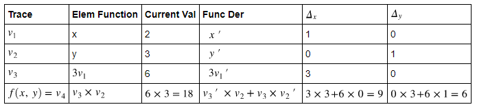
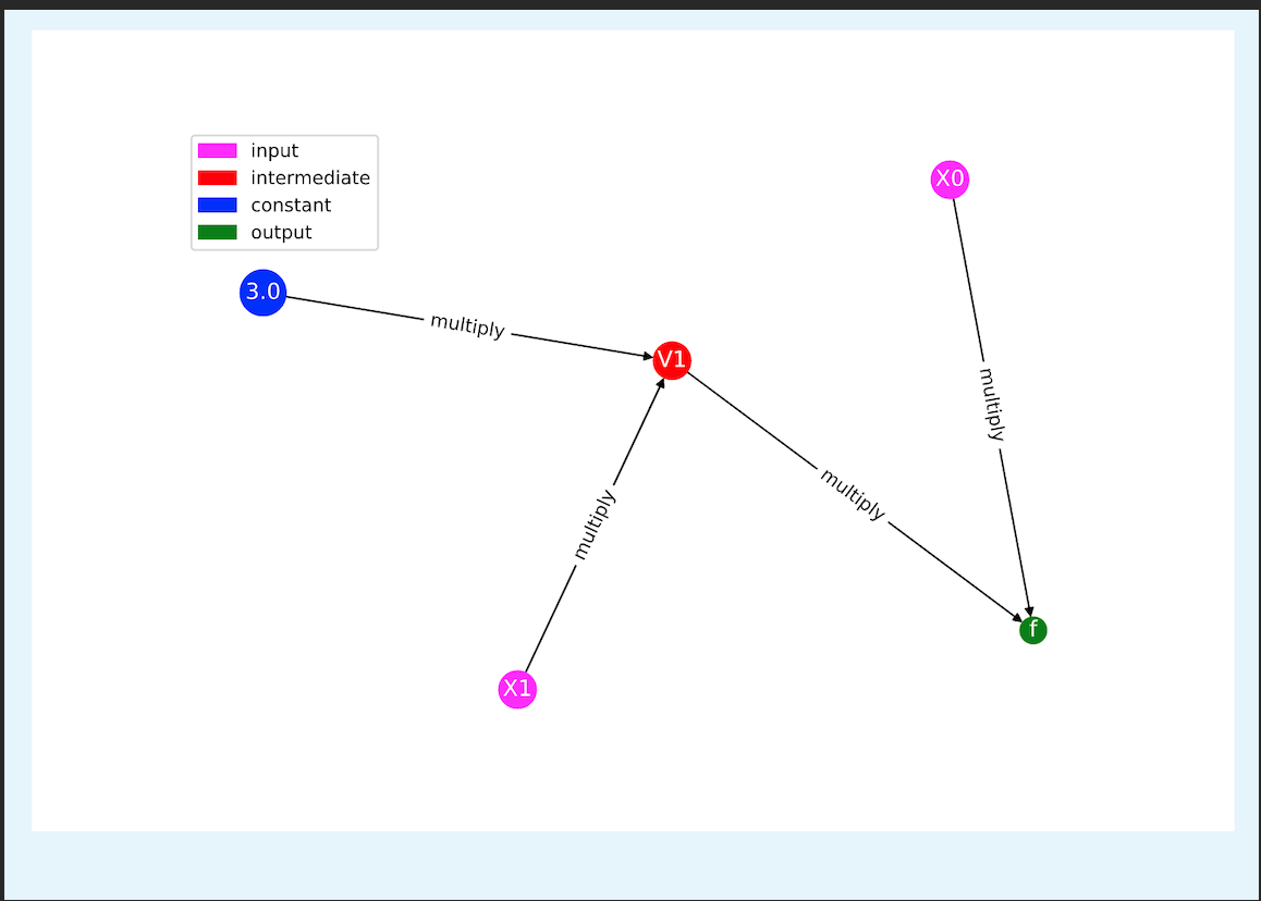
Example Trace Evaluation of Above Problem
$ v_1 = x = X_1$
$ v_2 = y = X_0$
$ v_3 = 3v_1 = V_1$
$ v_4 = f(x,y) = v_2 \times v_3 = f$
Software Organization
README.md
demos/                   Final Presentation with appropriate helper files
   Presentation.ipynb    Final Presentatoin
   ...
docs/                    Contains the documentation for the project.
   README.md
   documentation.ipynb   The main documentation.
   milestone1.ipynb
   milestone2.ipynb
   milestone2_progress.ipynb
   ...

code/                     Source files
   AADUtils.py              Utilities used as support functions (internal)
   AAD.py                   Main constructor and dual number forward-mode implementation=
   AADFunction.py           Vector-valued functions wrapper
   ...
   solvers/
      GradientDescent.py    Gradient-descent optimizer
      Newton.py             Newton root finder (vector-valued, linear and nonlinear functions)
      GMRES.py              Generalized Minimum-Residual Method root finder (vector-valued, linear functions)

tests/                   Contains the test suite for the project
   run_tests.py             Runs all of the tests it the folder
   test_funtion.py         Tests Vector Valued Functions of AD Variables
   test_gmres.py           Tests for GMRES
   test_graddesc.py        Tests for gradient descent
   test_main.py            Contains operations overrides and tests of complex functions for one variable
   test_newton.py          Tests for newton's method
   test_utils.py           Tests internal utilities
Implementation
Elementary Functions:
exp(x)euler's number to the power of xlog(x)natural log of xsin(x)sine of xsinh(x)hyperbolic sin of xcos(x)cosine of xcosh(x)hyperbolic cosine of xtan(x)tangent of xtanh(x)hyperbolic tangent of xarcsin(x)inverse sine of xarccos(x)inverse cosine of xarctan(x)inverse tangent of xsqrt(x)square root of x
Operation Overrides
__rmul__,__mul__,__neg__,__add__,__radd__,__sub__,__rsub____truediv__,__rtruediv__,__pow__,__rpow__,__repr__
These overrides accept real numbers, but do not assume real numbers. They can be used with multile AADVariable Objects
Thse overriden operators allow for seamless operations and combindations of operations that include:
- Power operations:
2**xorx**2 - Multiplication operations:
x*2or2*xorsin(x)*cos(x) - Negative operations:
x-3or3-xorsin(x)-cos(x) - Division operations:
x/4or4/xorsin(x)/cos(x) - Addition operations:
x+5or5+xorsin(x)+cos(x)
How to Use
Quick Initialization
git clonethis package repository into your project directory.- Install dependencies using
pip:pip install -r requirements.txt - Import our package using the following:
from AAD import as ADfor AAD objectsfrom AADFunction import as ADFfor vector valued functionsfrom solvers.Newton import AAD_Newtonfor Newton's Methodfrom solvers.GradientDescent import AAD_gradfor Gradient Descentfrom solvers.GMRES import AAD_GMRESfor GMRES
As a quick reference, you can install AAD with conda with a new environment using the following commands:
git clone git@github.com:dist-computing/cs107-FinalProject.git AAD
cd AAD
conda create --name AAD python=3.8
conda install -n AAD requirements.txt
To activate the environment later, simply use source activate AAD.
To install using PyPI via pip, AAD is the package namespace, and thus import is slightly different:
$ python -m pip install --upgrade aad-jimmielin

$ python
>>> from AAD.AADVariable import AADVariable
>>> x = AADVariable(1.0, [1,0])
>>> y = AADVariable(2.0, [0, 1])
>>> x*y
AADVariable fun = 2.0, der = [2. 1.]

>>> from AAD.AADFunction import AADFunction
>>> f = AADFunction([x+1, y*x])
>>> print(f)
[AADFunction fun = [2.0, 2.0], der = [[1. 0.]
 [2. 1.]]]
Github Pages Website Publishing
To efficiently publish the github pages website we further streamlined the work with bash scripting. In the script
included in the package a person can keep two folders with two branches, one for github pages and one for the gh-pages.
By running the bash script below, you can update the website based on the documentation file. ./UpdateIndexFromDocomentation.sh
#!/bin/bash

cd ../website/

#copy files from main repo
cp ../cs107-FinalProject/docs/documentation.ipynb ./documentation.ipynb

#convert notebook to markdown
jupyter nbconvert $(pwd)/documentation.ipynb --to markdown --output $(pwd)/index.md

#add title to file
sed -i '1s/^/---\n/' index.md
sed -i '1s/^/ title: About the code \n/' index.md
sed -i '1s/^/---\n/' index.md

#commit, push and publish
git add index.md documentation.ipynb
git commit -m 'updated index.md with documentation <automated>'
git push
Requirements & Dependencies
import sys
sys.path.insert(1, '../AAD/')
#importing Dependencies
import numpy as np
import AAD as AD
import AADFunction as ADF
import math
One Dimensional Example - simple case
Function & Evaluation
$ f(x) = \ln(x) $ at x = 4
$ f(x) = \ln(4) = 1.3862943611198906 $
Derivative & Evaluation
$ f'(x) = \frac{{1}}{x} $
$ f'(4) = \frac{{1}}{4} = 0.25 $
x = 4 #initial value of x

my_AD = AD.AADVariable(x) #creating the AAD object

my_AD = AD.log(my_AD) #applying a function to the object to find both the value and derivative

#Prints value of log and derivative at x = 4
print(my_AD)
AADVariable fun = 1.3862943611198906, der = 0.25
One Dimensional Example - Complex Case
Function & Evaluation
$ f(x) = e^{tan(x)}$ at x = $\pi$
$ f(\pi) = e^{tan(\pi)} = 1 $
Derivative & Evaluation
$ f'(x) = \frac{{1}}{cos^2(x)} \times e^{tan(x)} = \frac{{e^{tan(x)}}}{cos^2(x)}$
$ f'(\pi) = \frac{{e^{tan(\pi)}}}{cos^2(\pi)} = 1$
x = math.pi #initial value of x

my_AD = AD.AADVariable(x) #creating the AAD object

my_AD = AD.exp(AD.tan(my_AD)) #applying a function to the object to find both the value and derivative

#Prints value of e^tan(x) and derivative at x = pi
print(my_AD)
AADVariable fun = 0.9999999999999999, der = 0.9999999999999999
Multi Dimensional Example - simple case
Function & Evaluation
$ f(x,y) = x + y - 6 $ at x = 1.0 and y = 2.0
$ f(1,2) = 1.0 + 2.0 - 6 = - 3.0$
Partial Derivative with respect to X
$ \frac{\partial f}{\partial x} (x,y) = 1.0 $
$ \frac{\partial f}{\partial x} (1.0,2.0) = 1.0 $
Partial Derivative with respect to Y
$ \frac{\partial f}{\partial y} (x,y) = 1.0 $
$ \frac{\partial f}{\partial y} (1.0,2.0) = 1.0 $
Derivative Evaluation
$ f'(1.0,2.0) = \begin{bmatrix} 1.0 & 1.0 \end{bmatrix}$
### Multi Dimensional Example - simple case
x = AD.AADVariable(1.0, [1, 0]) # x = 1.0
y = AD.AADVariable(2.0, [0, 1]) # y = 2.0
scalar = 6.0

f = x + y - scalar

print(f)
AADVariable fun = -3.0, der = [1 1]
Advancing the Multidimensional Case - using previously declared AAD variables
Function & Evaluation
$ f(x,y) = \frac{x+ \frac{y}{2}}{10} $ at x = 1.0 and y = 2.0
$ f(1.0,2.0) = \frac{1.0+ \frac{2.0}{2}}{10} = 0.2$
Partial Derivative with respect to X
$ \frac{\partial f}{\partial x} (x,y) = 1.0/10 $
$ \frac{\partial f}{\partial x} (1.0,2.0) = 0.1 $
Partial Derivative with respect to Y
$ \frac{\partial f}{\partial y} (x,y) = 0.5/10 $
$ \frac{\partial f}{\partial y} (1.0,2.0) = 0.05 $
Derivative Evaluation
$ f'(1.0,2.0) = \begin{bmatrix} 0.1 & 0.05 \end{bmatrix}$
#Advancing Multi Dimensional using previously declared AAD Variables

print((x + 0.5*y)/10) # 0.1x+0.05y
AADVariable fun = 0.2, der = [0.1 0.05]
Multi Dimensional Example - Adding a Variable
Function & Evaluation
$ f(x,y,z) = x \times y \times z$ at x = 2.0, y = 1.0 and z = 4.0
$ f(2.0,1.0,4.0) = 2.0 \times 1.0 \times 4.0 = 8.0$
Partial Derivative with respect to X
$ \frac{\partial f}{\partial x} (x,y,z) = y \times z$
$ \frac{\partial f}{\partial x} (2.0,1.0,4.0) = 1.0 \times 4.0 = 4.0$
Partial Derivative with respect to Y
$ \frac{\partial f}{\partial y} (x,y,z) = x \times z $
$ \frac{\partial f}{\partial y} (2.0,1.0,4.0) = 2.0 \times 4.0 = 4.0 = 8.0$
Partial Derivative with respect to Z
$ \frac{\partial f}{\partial z} (x,y,z) = x \times y $
$ \frac{\partial f}{\partial z} (2.0,1.0,4.0) = 2.0 \times 1.0 = 2.0$
Derivative Evaluation
$ f'(2.0,1.0,4.0) = \begin{bmatrix} 4.0 & 8.0 & 2.0 \end{bmatrix}$
The AADVariable parser automatically zero-pads required derivative arrays, thus both of the following syntaxes work
### Multi Dimensional Example - complex case
x = AD.AADVariable(2.0, [1, 0, 0]) # x = 2.0
y = AD.AADVariable(1.0, [0, 1, 0]) # y = 1.0
z = AD.AADVariable(4.0, [0, 0, 1]) # z = 4.0

f = x*y*z
print(x*y*z)

x = AD.AADVariable(2.0, [1]) # x = 2.0
y = AD.AADVariable(1.0, [0, 1]) # y = 1.0
z = AD.AADVariable(4.0, [0, 0, 1]) # z = 4.0
print('We get the same result')

f = x*y*z
print(x*y*z)
AADVariable fun = 8.0, der = [4. 8. 2.]
We get the same result
AADVariable fun = 8.0, der = [4. 8. 2.]
Vector Valued Functions
Function & Evaluation
$f(x,y,z) = \begin{bmatrix} x+y \times z\\ z \times x-y \end{bmatrix}$ at x = 3.0, y = 2.0, and z=1.0*
$f(3.0,2.0,1.0) = \begin{bmatrix} 3.0+2.0 \times 1.0\\ 1.0 \times 3.0-2.0 \end{bmatrix} = \begin{bmatrix} 5.0\\ 1.0 \end{bmatrix} $
Partial Derivative with respect to X
$\frac{\partial f}{\partial x} (x,y,z) = \begin{bmatrix} 1.0\\ z \end{bmatrix}$
$\frac{\partial f}{\partial x} (3.0,2.0,1.0) = \begin{bmatrix} 1.0\\ 1.0 \end{bmatrix}$
Partial Derivative with respect to Y
$\frac{\partial f}{\partial y} (x,y,z) = \begin{bmatrix} z\\ -1.0 \end{bmatrix}$
$\frac{\partial f}{\partial y} (3.0,2.0,1.0) = \begin{bmatrix} 1.0\\ -1.0 \end{bmatrix}$
Partial Derivative with respect to Z
$\frac{\partial f}{\partial Z} (x,y,z) = \begin{bmatrix} y\\ x \end{bmatrix}$
$\frac{\partial f}{\partial Z} (3.0,2.0,1.0) = \begin{bmatrix} 2.0\\ 3.0 \end{bmatrix}$
Derivative Evaluation
$ f'(2.0,1.0,4.0) = \begin{bmatrix} 1.0 & 1.0 & 2.0\\ 1.0 & -1.0 & 3.0 \end{bmatrix}$
x = ADF.AADVariable(3.0, [1]) # either not specifying der, [1], or [1 0] or [1,0,0] will all work, as above
y = ADF.AADVariable(2.0, [0, 1])
z = ADF.AADVariable(1.0, [0, 0, 1])

f_1 = x+(y*z)
f_2 = (z*x)-y
f = ADF.AADFunction([f_1, f_2])
print(f)
[AADFunction fun = [5.0, 1.0], der = [[ 1.  1.  2.]
 [ 1. -1.  3.]]]
Added Feature (Root Finder): Newton's Method, GMRES, & Gradient Descent
GMRES
uses
AAD's automatic differentiation core to solve systems of linear equations.Given a system of $k$ linear equations for the function $F: \mathbb{R}^k \rightarrow \mathbb{R}^k$ with a nonsingular Jacobian matrix $J_F(x_n)$
- Iteratively solve by applying the GMRES solver to the action of the operator $F$ on a seed vector $v$, to yield $\Delta x_k$ for the next iteration.
Is all that is needed for GMRES to solve for $J_F(x_k)\Delta x_{k} = -F(x_k)$, and thus does not require the computation of the Jacobian itself.
Using this principle we can iteratively solve for $\Delta x_k$ and improving the guess until convergence.
#GMRES
x = AD.AADVariable(3, [1 ,0])
initial_guess = [30]
solve = AAD_GMRES.solve(lambda x: [3*x-2], initial_guess)
print(solve[0])
0.6666666666666679
Newton's Method
- uses the
AAD's automatic differentiation core to solve systems of linear and non-linear equations. - solves or a system of $k$ (nonlinear)equations and continuously differentiable function $F: \mathbb{R}^k \rightarrow \mathbb{R}^k$
- we have the Jacobian matrix $J_F(x_n)$ yielding
Inverting the Jacobian is expensive and unstable
solving the following linear system is more practical:
We implement this using our automatic differentiation core, which retrieves the Jacobian $J_F(x_n)$ accurate to machine precision
In the future we can also expand Newton's Method solver to a "least squares sense" solution problem by using a generalized inverse of a non-square Jacobian matrix $J^\dagger = (J^TJ)^{-1}J^T$ for non-linear functions, thus expanding our optimization toolbox.
#Newton's Method
x = AD.AADVariable(3, [1 ,0])
initial_guess = [30]
solve = AAD_Newton.solve(lambda x: [3*x-2], initial_guess)
print(solve)
[0.6666666666666666]
Gradient Descent
- Uses the gradient to minimize the function and follow the descent of the funciton topology.
- Updates the location and obtaining the gradient at that location of the function namely:
Where $a_{n+1}$ is the new point based on the previous point $a_n$ updated by the gradient of the function evaluated at the previous point $$\gamma\nabla F(a_n)$$, where $$\gamma$$ provides the step size.
#Gradient Descent
x = AD.AADVariable(3, [1 ,0])
gamma = .0001
solve = AAD_grad.solve(lambda x: AD.abs(3*x[0]-2), [x], gamma)
print(solve[0].val)
0.6665999999995169
Concluding Sections
Broader Impact & Inclusivity
- We have a diverse interdisciplinary team
- Lived experience and cultural background
- Academic background - environmental sciences, engineering, and public policy
- Code was assessed by all group members and also inlcuded genuine and vulnerable group discssion
- Our team would HIGHLY benefit from contribution from women - the first and most important addition we see moving forward
- Inclusivity and impact are never fnished
- We will keep flexible and open minds to continue thinking about how are software can be improved both in it's quantitative power and who it effects.
Future Features & Ideas
Reverse Mode
- implement the reverse mode scheme of automaotic differentiation. Having this toolset in addition to optimizers is extremely valuable in the field of AI as it allows one to efficiently compute the backwardpropagation of errors in multilayer perceptions (i.e. neural networks).
The implementation of backwardpropagation of neural networks is essnetiall a special case of reverse mode AD with an added set of elementary functions. These elementary functions are called activation functions some of which are already implemented in this version of the software.
Here is a comprehensive list of new and already implemented functions we plan on incorporating into the future version of this software.
New Functions: relu, leaky relu, sigmoid, swish, softmax, binary step
Already implemented: linear, tanh
Optimizers
- Add personalized optimizers and root finders
- Users can define their own algorithm and compare to other models
- Create a visualization tool set where users are able to compare the training, testing, and timing performce of their code
- Compares to the built in optimizatio/root-finding algorithm.
In Summation
Background & Introduction
- comprehensive and mathematically sound
Implementation/Software Organization/How to Use
- Intitutive for users in terms of structure and outward facing functions
- Offering a variety of features that can be accessed in multiple ways
Additional Features/Extension
- Groundwork for optimiziation
- Fully functioning tool set that has a variety of options for comparison
Impact and Inclusivity
- A diverse team with positive intentions
- Can always be improved
Future Work & Other Possible Extensions
- Enhanced methods of optimization that build on our codebase intuitively
We appreciate your time and patience watching this presentation. We hope it has been informative. Please Email us with any questions - we will respond promptly.
benjaminmanning@hks.harvard.edu
fernandes@g.harvard.edu
hplin@g.harvard.edu