Awesome Automatic Differentiator
Project maintained by:
- Matheus C. Fernandes
- Heipeng Lin
- Benjamin Manning Hosted on GitHub Pages — Theme by mattgraham
Done as partial fullfilment for Harvard CS107/AC207
Thanks to Jonathan Jiang and Prof. David Sondak!
Final Project Presentation Video
Slides Deck
Please find the slide deck from the presentation in this link
aad.fer.me/Presentation.slides.html
Introduction
This software solves the issue of accurate differentiation. Accurate differentiation is important for many fields such as machine learning, numerical methods and optimization. Being able to accuratelly know the derivative of a non-linear function allows programers and mathematicians to quickly take derivatives when the focus of their research or project does not rely on the actual steps of differentiating a function, but simply finding the correct answer for the derivative of a given equation to move forward in their work.
Unlike finite-difference numerical differentiation which is an approximation, automatic differentiation uses dual numbers to compute within machine precision exact derivatives based on elementary primitives, allowing for high-performance and highly accurate computation of numerical derivatives, which are useful for many fields.
This software package will do just that for N number of variables and complex derivatives that would otherwise be extremely challenging to evaluate. This process should help minimize errors as compared to numerical methods.
Background
The main mathematical idea behind automatic differentiation is to break downs the process of differentiation into specific and iterable steps. We do so by breaking down each equation into to elementary arithmetic operations such as addition, subtraction, multiplication, division, power, expoential, logarithmic, cos, sin, tan, etc. To perform this process, automatic differentiation uses the power of the chain rule to brake down derivatives of composit functions into easily solvable components. The benefit of following this approach is that it allows the derivative evaluation to be as accurate as possible up to computer precision, unlike numerical differentiation.
Automatic differentiation is benefitial because it can be used in two ways. The forward and the reverse accumulation. The workings of each of the two modes are described in more detail below.
Forward Accumulation
In this mode we break down the equation by following chain rule as we would when doing it by hand. This approach is benefitial to compute accurate differentiation of pf matrix producs such as Jacobians. Because AD method inherently keeps track of all operations in a table, this becomes very efficient for evaulation other types higher order derivative based matrices such as Hessians.
Reverse Accumulation
In this mode, the dependent variable is fixed and the derivative is computed backward recursively. This means that this accumulation type travels through the chainrule in a backward fashion, namely, from the outside toward the inside. Because of its similarity to backpropagation, namely, backpropagation of errors in multilayer perceptrons are a special case of reverse mode, this type of computational coding is a very efficient way of computing these backpropagations of error and ultimatly enables the ability to optimize a the weights in a neural network.
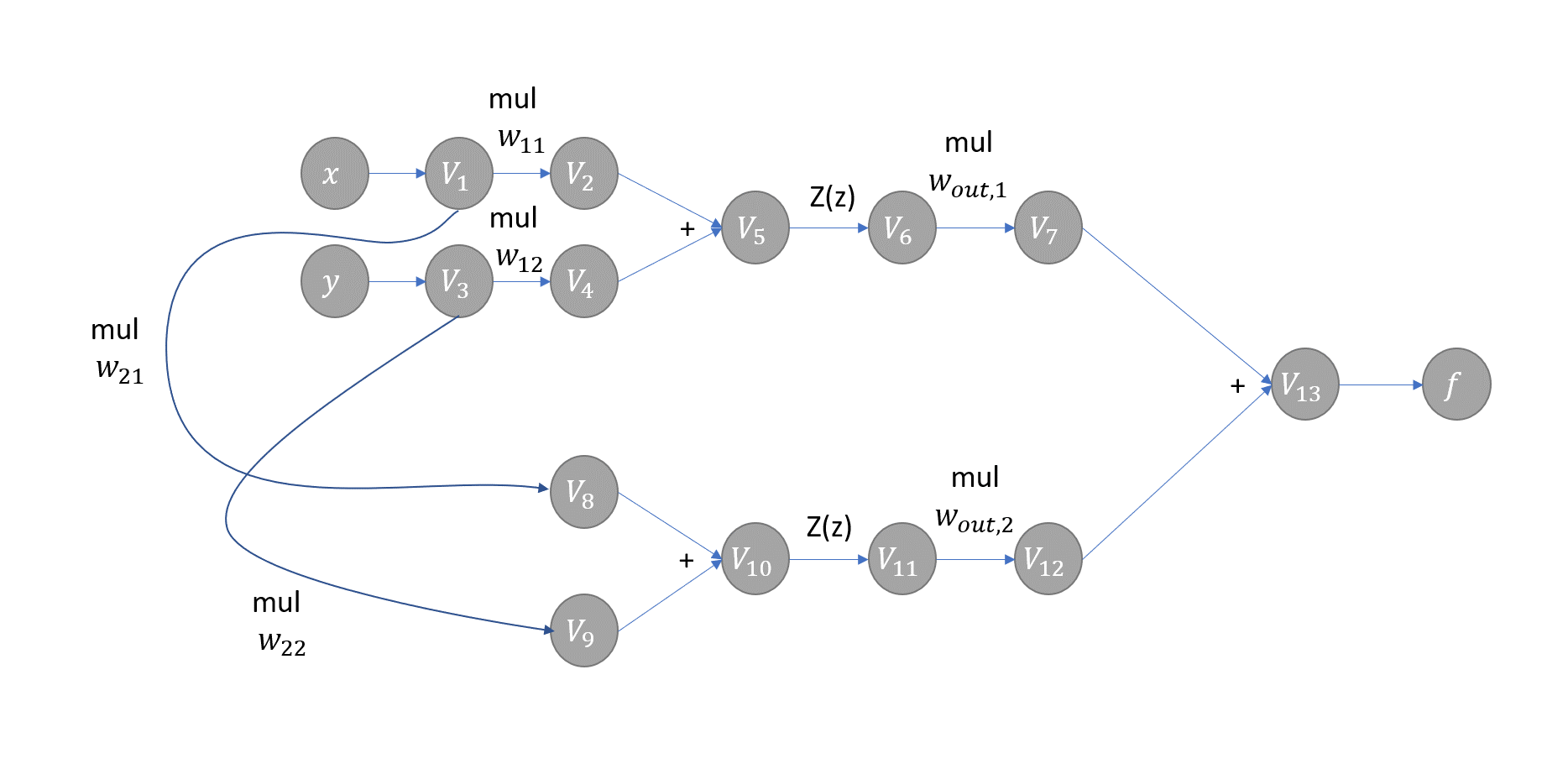
Example Evaluation Trace for a Simple Neural Network
How to use AAD (“Awesome Automatic Differentiation”)
Quick Initialization
git clonethis package repository into your project directory.- Install dependencies using
pip:pip install -r requirements.txt - Import our package using the following:
from AAD import as ADfor AAD objectsfrom AADFunction import as ADFfor vector valued functionsfrom solvers.Newton import AAD_Newtonfor Newton’s Methodfrom solvers.GradientDescent import AAD_gradfor Gradient Descentfrom solvers.GMRES import AAD_GMRESfor GMRES
- Run the tests; either using
pytestor the manual test python script atpython ./tests/run_tests.py. - Consult the documentation for quick examples to get started.
How to Install using Conda to create an environment
It is good practice to use virtual environments (such as Anaconda) to prevent tampering with your existing package installation in python.
As a quick reference, you can install AAD with conda with a new environment using the following commands:
git clone git@github.com:dist-computing/cs107-FinalProject.git AAD
cd AAD
conda create --name AAD python=3.8
conda install -n AAD requirements.txt
To activate the environment later, simply use source activate AAD.
How to install as a package from pip
If you prefer the distribution to be installed using PyPI, then install the aad-jimmielin package:
pip install aad-jimmielin
Import package contents from the AAD. package namespace using:
from AAD.AADVariable import AADVariable
An interactive example:
$ python -m pip install --upgrade aad-jimmielin
Collecting aad-jimmielin
  Downloading aad_jimmielin-1.1.1-py3-none-any.whl (7.3 kB)
Successfully installed aad-jimmielin-1.1.1

$ python
Python 3.7.9 (default, Oct 13 2020, 21:10:49)
[GCC 8.3.0] on linux
Type "help", "copyright", "credits" or "license" for more information.
>>> from AAD.AADVariable import AADVariable
>>> x = AADVariable(1.0, [1,0])
>>> y = AADVariable(2.0, [0, 1])
>>> x*y
AADVariable fun = 2.0, der = [2. 1.]

>>> from AAD.AADFunction import AADFunction
>>> f = AADFunction([x+1, y*x])
>>> print(f)
[AADFunction fun = [2.0, 2.0], der = [[1. 0.]
 [2. 1.]]]
>>>
Code example (univariate)
You can create a driver script at the top level, e.g. my_code.py, and include the following code to use the AAD package:
import AAD as AD
import math
#Evaluate the derivative of log(x) at x = 4
x = 4 #initial value of x
my_AD = AD.AADVariable(4) #creating the AAD object
my_AD = AD.log(my_AD) #applying a function to the object to find both the value and derivative
#Prints value of log and derivative at x = 4
print(my_AD)
Answer:
AADVariable fun = 1.3862943611198906, der = 0.25
Toy implementation of Newton’s Method
You can retrieve the Jacobian (or scalar derivative) by tapping into the .der attribute of the AAD, or using the .jacobian() function on a AADVariable object.
With this you can solve for roots on functions, with the Newton’s Method, i.e. for sin(x):
# Newton's Method for solving root (toy implementation, we have a better one!)
# of f(x) = sin(x)
x0 = AADVariable(2.0)
for i in range(1, 20): # do 20 iterations maximum
    fx = sin(x0)
    x1 = x0.val - fx.val/fx.der
    if abs(x0.val - x1) > 10e-6: # larger than minimum tolerance?
        x0 = AADVariable(x1)
    else:
        break
print(x0.val) # Final solution
This prints
3.1415926536808043
Advanced Examples
Multivariate usage
AAD fully supports vector-based inputs and outputs for its functions. For vector inputs, variables are not named but instead identified by a positional vector (“seed vector”).
We believe this implementation is more flexible and allows for arbitrary number of input components with a clear mathematical meaning.
Multiple variables are communicated to the AADVariable dual number class using the second argument (derivative der) as a vector, i.e.
[1, 0] is the first variable, [0, 1] is the second. Of course, specifying (x+y) as a composite variable using [1, 1] is also supported.
A two-variable example:
x = AADVariable(1.0, [1, 0]) # x = 1.0
y = AADVariable(2.0, [0, 1]) # y = 2.0
scalar = 6.0

print(x + y - scalar) # AADVariable fun = -3.0, der = [1 1]
print(x * y - scalar) # AADVariable fun = -4.0, der = [2. 1.]
print((x + 0.5*y)/10) # 0.1x+0.05y, AADVariable fun = 0.2, der = [0.1  0.05]
As you can see, each indexed entry in the derivative correspond to the partial derivative with respect to that variable.
How can I add more variables? The code is flexible and enables adding more variables without changing the previous seed vectors. e.g. the following will work:
x = AADVariable(1.0, [1, 0]) # x = 1.0
y = AADVariable(2.0, [0, 1]) # y = 2.0
z = AADVariable(9.0, [0, 0, 1]) # z = 9.0
print(x*y*z) # AADVariable fun = 18.0, der = [18.  9.  2.]
The AADVariable parser automatically zero-pads required derivative arrays, thus the following will work just fine:
x = AADVariable(1.0, [1]) # x = 1.0
y = AADVariable(2.0, [0, 1]) # y = 2.0
z = AADVariable(9.0, [0, 0, 1]) # z = 9.0
For compatibility, if only one variable is detected, all values are returned as scalars, otherwise they return a np.ndarray.
Vector-valued functions - the AADFunction class
For vector valued functions, they need to be wrapped in the AADFunction class to be tracked correctly. An example:
x = AADVariable(1.0, [1]) # either not specifying der, [1], or [1 0] or [1,0,0] will all work, as above
y = AADVariable(2.0, [0, 1])
f = AADFunction([x+y, x-y])
print(f)
This prints:
[AADFunction fun = [3.0, -1.0], der = [[ 1  1]
 [ 1 -1]]]
Where you can see that the Jacobian is [1 1; 1 -1]. The value and the derivative are retrieved from f.val() and f.der() methods, respectively.
How to use AAD’s Optimization and Solver Suite
AAD includes an awesome set of optimizers and solvers for scalar and vector-valued functions, including:
Newton’s method for finding roots. Usable for linear and non-linear scalar or vector-valued functions.GMRES(generalized minimal residual method) for finding roots. Used for linear scalar or vector-valued functions.- A
GradientDescentoptimizer.
Examples
Gradient Descent Optimizer
To optimize using the Gradient Descent optimizer, specify the function using def Function(X): where X is a vector composed
of the different variables. If the function only contains one variable X should be a vector with only one entry. Note that the
initial values also must be a vectored list with the same dimensions as the function.
import AAD as AD
from solvers.GradientDescent import AAD_grad
x = AD.AADVariable(3, [1 ,0])
y = AD.AADVariable(2, [0, 1])

solve = AAD_grad.solve(lambda X: AD.abs(2*X[0]-12+2*X[1]**2),[x,y],0.001,progress_step=5000,max_iter=10000)
Newton’s method root solver
To solve roots using Newton’s Method, simply specify the functions using Python’s lambda function features.
from solvers.Newton import AAD_Newton
print(AAD_Newton.solve(lambda x, y, z, a: [x+4*y-z+a, a-2, y*5+z*0.1, x+2*a], [1, 1, 1, 1])) # [-4.0, 0.03703703703703704, -1.851851851851852, 2.0]
print(AAD_Newton.solve(lambda x: [x*y+1, 3*x+5*y-1], [1])) # two sets of roots; the one solved here is [-1.1350416126511096, 0.8810249675906657]; depends on initial guess
What’s happening under the hood?
- The lambda function is translated to a set of
AADVariablemulti-variate inputs. We use lambda functions so we can have “faux” symbolic math and it looks pretty. - The function results are wrapped in
AADFunctionand automatically differentiated. - Newton’s method is used to solve the equation.
GMRES
GMRES only works for linear functions. The method signature is similar to the Newton’s method above:
from solvers.GMRES import AAD_GMRES
print(AAD_GMRES.solve(lambda x, y: [x+y+5, 3*x-y+1], [0.5, 1.5])) # [-1.5, -3.5]
print(AAD_GMRES.solve(lambda x: [x-2], [300])) # [2.0]
Organization
Directory structure and modules
- We will have a main importable class that contains the directions for each function and how to use them.
README.md
demos/                   Final Presentation with appropriate helper files
   Presentation.ipynb    Final Presentatoin
   ...
docs/                    Contains the documentation for the project.
   README.md
   documentation.ipynb   The main documentation.
   milestone1.ipynb
   milestone2.ipynb
   milestone2_progress.ipynb
   ...
code/                     Source files
   AADUtils.py              Utilities used as support functions (internal)
   AAD.py                   Main constructor and dual number forward-mode implementation=
   AADFunction.py           Vector-valued functions wrapper

   solvers/
      GradientDescent.py    Gradient-descent optimizer
      Newton.py             Newton root finder (vector-valued, linear and nonlinear functions)
      GMRES.py              Generalized Minimum-Residual Method root finder (vector-valued, linear functions)

tests/                   Contains the test suite for the project
   run_tests.py             Runs all of the tests it the folder
   test_funtion.py         Tests Vector Valued Functions of AD Variables
   test_gmres.py           Tests for GMRES
   test_graddesc.py        Tests for gradient descent
   test_main.py            Contains operations overrides and tests of complex functions for one variable
   test_newton.py          Tests for newton's method
   test_utils.py           Tests internal utilities
Modules
- The modules that we will use are
numpy,math,SimPy,SciPynumpywill be used in order to evaluate and analyze arrays.mathwill be used in for its access to simple mathematical functions.SimPywill potentially be used to take symbolic derivatives and will be useful in our test suite. Additionally, if a function is not in our elementary functions, we can use this module to help evaluate them.SciPywill be useful to test how our automatic differentiator compares to numeric derivatives (speed test).
Test suite
- Our test suite will live inside the
testsfolder within our main repository.- The tests cover all elementary functions, including overloaded operators (
__add__,__mul__, etc.) and trigonometric functions (sin,arccos, …) and other functions (log,sqrt)- This also includes covering vector valued functions for similar examples
- Both the values and the derivatives generated by
AAD’s forward mode are compared to analytical solutions. - Our tests cover all three root solvers with single variable and multi-variable examples
- The tests cover all elementary functions, including overloaded operators (
- The
run_tests.pyfile runs all tests in our suite to make sure software works effectively for given coverage. - We will use
TravisCIto test our suite. View CI test results here. - Our Coverage on
Codecovcan be found here. We always maintain above 90% coverage. [View Coverage Here] (https://codecov.io/gh/dist-computing). - You can also manually run tests using
pytestto ensure your installation and environment is correct.
Implementation
Data structures
The AAD class holds dual numbers and elementary functions required to perform algebra with dual numbers. The dual number
class is AADVariable supporting scalar and vector inputs, and vector valued functions are supported by a AADFunction
auxiliary type.
Internal data structures include the numpy.ndarray data type and number types.
Classes and method signatures
The AAD dual number class
This is a single variable dual number with forward-mode automatic differentiation. Includes representation and string functions, i.e. __repr__ and __str__.
Allows retrieval of the function value (i.e. .val) and derivative (scalar “jacobian”) value (i.e. .der).
The AAD class
Includes APIs used for performing Automatic Differentiation, as of the current version, AAD can handle single varibale differentiation that include terms using the following elementary functions:
exp(x)euler’s number to the power of xlog(x)natural log of xsin(x)sine of xsinh(x)hyperbolic sin of xcos(x)cosine of xcosh(x)hyperbolic cosine of xtan(x)tangent of xtanh(x)hyperbolic tangent of xarcsin(x)inverse sine of xarccos(x)inverse cosine of xarctan(x)inverse tangent of xsqrt(x)square root of x
Additionally, the Jacobian can be returned through calling its method:
x.jacobian()– returns the jacobian of the AADVariable Object.
Attributes
Our classes will have the following attributes
__init__(val, der 0, name = none)– initialization and all variables where val is the value, der is the derivative and name is the name of the variable.der– provides the derivative of the function at the original point.val– provides the value of the function at the original point.name– used for future upgrades to software
External dependencies
For matrix support, this software package requires numpy, math, SimPy, SciPy.
Vector Valued Functions
For these functions we will evaluate each element of the vector valued function independently and then move on to the next element. We will store each evaluation in a numpy array - akin to a jacobian to output the correct derivative.
Elementary Operators
We will overload the addition, multiplication, subtraction, division, and power operators to work within our software using the baseline dunder methods and the reverse versions.
The Following Elementary Operators have been overriden:
__rmul__,__mul__,__neg__,__add__,__radd__,__sub__,__rsub____truediv__,__rtruediv__,__pow__,__rpow__,__repr__
These overrides accept real numbers, but do not assume real numbers. They can be used with multile AADVariable Objects
Thse overriden operators allow for seamless operations and combindations of operations that include:
- Power operations:
2**xorx**2 - Multiplication operations:
x*2or2*xorsin(x)*cos(x) - Negative operations:
x-3or3-xorsin(x)-cos(x) - Division operations:
x/4or4/xorsin(x)/cos(x) - Addition operations:
x+5or5+xorsin(x)+cos(x)
Elementary functions
Elementary functions are implemented using built-in Python math and the numpy package and include ready-made implementations for Dual numbers in this package.
To deal with elementary functions such as sin, log and exp we will manually evaluate them and add them to a database to query continuously using the chain rule.
- The derivative of
sin(x)=x' * cos (x) - The derivative of
log(x)=x' * 1/x - The derivative of
exp(x)=x' * exp(x)
Additionally, for other all other functions in the AAD class we perform the same process, with the chain rule.
New Feature
Newton’s Method
The Newton’s Method solver uses the AAD’s automatic differentiation core to solve systems of linear and non-linear equations. For a system of $k$ (nonlinear)
equations and continuously differentiable function $F: \mathbb{R}^k \rightarrow \mathbb{R}^k$ we have the Jacobian matrix $J_F(x_n)$ yielding
Inverting the Jacobian is very expensive and numerically unstable, thus solving the following linear system is more practical:
\[J_F(x_n)(x_{n+1}-x_n) = -F(x_n)\]We implement this using our automatic differentiation core, which retrieves the Jacobian $J_F(x_n)$ accurate to machine precision - this is the power of automatic differentiation!
In the future we can also expand Newton’s Method solver to a “least squares sense” solution problem by using a generalized inverse of a non-square Jacobian matrix $J^\dagger = (J^TJ)^{-1}J^T$ for non-linear functions, thus expanding our optimization toolbox.
Gradient Descent
The Gradient Descient optimizer uses the power of AAD’s automatic diferentiation core to efficiently and accurately solve
the gradient of the multi-variate function. It uses the gradient to minimize the function and follow the descent of the funciton
topology. It does that by updating the location and obtaining the gradient at that location of the function namely:
Where $a_{n+1}$ is the new point based on the previous point $a_n$ updated by the gradient of the function evaluated at the previous point \(\gamma\nabla F(a_n)\), where \(\gamma\) provides the step size.
GMRES
The GMRES (generalized minimal residual method) solver uses AAD’s automatic differentiation core to solve systems of linear equations.
When given a system of $k$ linear equations for the function (i.e. linear operator) $F: \mathbb{R}^k \rightarrow \mathbb{R}^k$ with a nonsingular Jacobian matrix $J_F(x_n)$, we can iteratively solve by applying the GMRES solver to the action of the operator $F$ on a seed vector $v$, to yield $\Delta x_k$ for the next iteration. Essentially
\[a = J_F(x_n) v\]Is all that is needed for GMRES to solve for $J_F(x_k)\Delta x_{k} = -F(x_k)$, and thus does not require the computation of the Jacobian itself.
Using this principle we can iteratively solve for $\Delta x_k$ and improving the guess until convergence.
Use Cases
\[f(x) = 3x-2\] \[0 = 3x-2\] \[0 = 3x-2\] \[2/3 = x\]
from solvers.Newton import AAD_Newton
from solvers.GradientDescent import AAD_grad
from solvers.GMRES import AAD_GMRES

#Newton's Method
x = AD.AADVariable(3, [1 ,0])
initial_guess = [30]
solve = AAD_Newton.solve(lambda x: [3*x-2], initial_guess)
print(solve) #this prints [0.6666666666666666]

#Gradient Descent
x = AD.AADVariable(3, [1 ,0])
gamma = .0001
solve = AAD_grad.solve(lambda x: AD.abs(3*x[0]-2), [x], gamma)
print(solve[0].val) #this prints [0.6666666666666666]

#GMRES
x = AD.AADVariable(3, [1 ,0])
initial_guess = [30]
solve = AAD_GMRES.solve(lambda x: [3*x-2], initial_guess)
print(solve[0]) #this prints [0.6666666666666666]
Broader Impact & Inclusivity Statement
For the Awesome Automatic Differentiation project, we had a diverse team of individuals from a variety of backgrounds contribute to all parts of the codebase. Our team brought in a diverse set of perspectives not only from our lived experience - which is essential to assessing inclusivity, but from an academic sense of diversity. For lived experience we come from three different countries and have lived in a variety of urban and rural settings. Additionally our team speaks multiple languages that we can use in order to communicate with external parties who want to work with us. Academically, we work in environmental sciences, applied mathematics and public policy, which has allowed our interdisciplinary team to assess the impact of our work from a variety of perspecitives - both ethical and quantitative. In the process of approving pull requests and assessing code, each member of our time approved all parts of the work through intensive reading and discussion, which allowed our disparate academic lenses to assess the strengths and weaknesses of our work. No decisions were made by just one person. Because of the diversity of perspective of our team, we believe our code is accessible to the vast majority of people. In the future, however, we would hope to add a female perspective to our code review and work, as we were assigned an all male team. This was a glaring weakness of our team that we were unable to fix, but will moving forward. We recognize that this could be a barrier to women using our code - so we will try to fix it by diversifying our team
We plan to publish our code as open source - which comes with a variety of risks. We cannot explicitly control the parties that use our code, but we will have public warnings attached to the documentation in the future. We recognize that individuals performing computation projects with nefarious and descriminatory goals (either knowlingly or unknowingly) could access our work. We will work to make sure that they are not contributing to our code base through assesssing of previous work and character before approval.
We want people to use our software as a tool for good - no matter what the projects. A final step that we believe is essential to propogating this subjective ‘good’ is for other teams to write impact statements. We see this as a superb practice in self-reflection, and before improving external contributions, we would want to see impact and inclusivity statements. However, if there’s were for some reason triggering to write for an individual, we would make ecxeptions.
In summation, we have worked to make this software inclusive with positive impact. However, inclusivity and impact are never complete. We will keep flexible and open minds to continue thinking about how are software can be improved both in its quantitative power and who it effects.
Future Features & Ideas
As an additional extension of this project, we would like to implement the reverse mode scheme of automaotic differentiation. Having this toolset in addition to optimizers is extremely valuable in the field of AI as it allows one to efficiently compute the backwardpropagation of errors in multilayer perceptions (i.e. neural networks). Being able to try different optimization schemes in addition to backward propogation will be useful in order to test the efficiency of different implementations. The implementation of backwardpropagation of neural networks is essnetiall a special case of reverse mode AD with an added set of elementary functions. These elementary functions are called activation functions some of which are already implemented in this version of the software. Here is a comprehensive list of new and already implemented functions we plan on incorporating into the future version of this software.
New Functions: relu, leaky relu, sigmoid, swish, softmax, binary step
Already implemented: linear, tanh
Furthermore, as an additional step in this project, we would like to propose creating a framework for adding personalized optimizers and root finders so that users can define their own algorithm and test its performance with other algorithms for a particular reverse mode neural network. We would like to also create a vizualization toolset where users are able to compare the training, testing, and timing performce of their code in comparison to the built in optimizatio/root-finding algorithm. This will give the users an idea of what would be the best scheme for their particular application.